Cactus Code

WaveToy Demo

Connect to our Cactus Demo to see the simple WaveToy example in action.

Setting up the WaveToy Demo

On this page we describe one of our standard demonstrations, which includes various tools which can be used with your own application, including

Compiling and running a simple Cactus application
Remote monitoring and steering of an application from any web browser
Streaming of isosurfaces from a simulation, which can then be viewed on a local machine
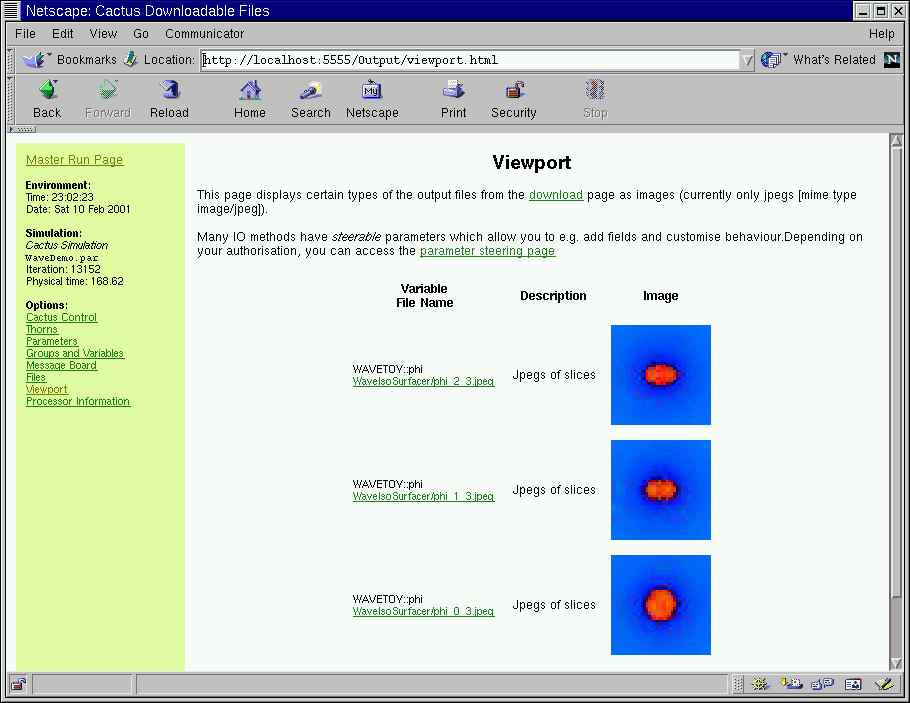
Remote visualization of 2D slices from any grid function in a simulation as jpegs in a web browser

This is a good example for you to try out yourself if you are trying out Cactus for the first time, or haven't used some of these tools before. Note that you only need a C compiler for this, and about 50MB of free diskspace.

The application we are using is the simulation of the 3D scalar field produced by two orbiting sources. The solution is found by finite differencing a hyperbolic partial differential equation for the scalar field. This is a very simple application, however it is representative of a large class of more complex systems, including Einstein's Equations, Maxwell's Equations, or the Navier-Stokes Equations. We use it for demonstrations since the simulation is not computationally intensive, is very robust, has simple parameter choices, and has reasonable graphics.

We are not going to describe completely here how to checkout and compile this Cactus application ... for this see the information on the Download page, the HOWTOs or the Users Guide. We assume that you are checking out Cactus using CVS, and that you know the configuration line needed, or have a configuration file, for compiling Cactus --- but even if you don't have a go, hopefully the default configuration will work for you!

Demo with Web Server and Streaming IsoSurfaces

Check out and compile

Checkout the source code using the GetComponents script. wget http://www.cactuscode.org/download/GetComponents chmod 755 GetComponents ./GetComponents http://www.cactuscode.org/documentation/tutorials/wavetoydemo/WaveDemo.th

Once the checkout has completed, move into the Cactus directory and compile the application. cd Cactus gmake WaveDemo-config gmake WaveDemo Hopefully that went OK, and you now have an executable, exe/cactus_WaveDemo. Check it really worked by running the testsuites, just type gmake WaveDemo-testsuite and use the default answers to each question.

Run the demo

Download the demo parameter file wget http://www.cactuscode.org/documentation/tutorials/wavetoydemo/WaveDemo.par

To start the simulation, run your new executable with the demo parameter file, if you have a single processor executable ./exe/cactus_WaveDemo WaveDemo.par

If you compiled with MPI and have a multiprocessor version, you will need to use the appropriate mpi command for running.

When the simulation starts, you will see output describing for example the activated thorns and the scheduling tree. tg-c305 dstark/Cactus> ./exe/cactus_WaveDemo parfiles/WaveDemo.par -------------------------------------------------------------------------------- 10 1 0101 ************************ 01 1010 10 The Cactus Code V4.0 1010 1101 011 www.cactuscode.org 1001 100101 ************************ 00010101 100011 (c) Copyright The Authors 0100 GNU Licensed. No Warranty 0101 -------------------------------------------------------------------------------- Cactus version: 4.0.b15 Compile date: Nov 19 2004 (08:52:01) Run date: Nov 19 2004 (08:54:30) Run host: tg-c305.ncsa.teragrid.org Executable: /home/ac/dstark/Cactus/./exe/cactus_WaveDemo Parameter file: parfiles/WaveDemo.par -------------------------------------------------------------------------------- Activating thorn Cactus...Success -> active implementation Cactus Activation requested for --->coordbase symbase pugh pughslab pughreduce isosurfacer iojpeg jpeg6b ioutil ioascii iobasic time wavetoyc cartgrid3d boundary idscalarwavec wavebinarysource httpd httpdextra socket<--- Activating thorn boundary...Success -> active implementation boundary Activating thorn cartgrid3d...Success -> active implementation grid Activating thorn coordbase...Success -> active implementation CoordBase Activating thorn httpd...Success -> active implementation HTTPD Activating thorn httpdextra...Success -> active implementation http_utils . . . Activating thorn wavebinarysource...Success -> active implementation binarysource Activating thorn wavetoyc...Success -> active implementation wavetoy -------------------------------------------------------------------------------- if (recover initial data) Recover parameters endif Startup routines [CCTK_STARTUP] CartGrid3D: Register GH Extension for GridSymmetry CoordBase: Register a GH extension to store the coordinate system handles GROUP HTTP_Startup: HTTP daemon startup group HTTPD: Start HTTP server GROUP HTTP_SetupPages: Group to setup stuff which needs to be done between starting the server and the first time it serves pages HTTPD: Serve first pages at startup HTTPDExtra: Utils for httpd startup PUGH: Startup routine IOUtil: Startup routine IOJpeg: Startup routine IOASCII: Startup routine IsoSurfacer: Startup routine IOBasic: Startup routine PUGHReduce: Startup routine SymBase: Register GH Extension for SymBase WaveToyC: Register banner . . . Termination routines [CCTK_TERMINATE] IsoSurfacer: Termination routine PUGH: Termination routine Shutdown routines [CCTK_SHUTDOWN] HTTPD: HTTP daemon shutdown Routines run after restricting: [CCTK_POSTRESTRICT] WaveToyC: Boundaries of 3D wave equation GROUP WaveToyC_ApplyBCs: Apply boundary conditions GROUP BoundaryConditions: Execute all boundary conditions Boundary: Apply all requested local physical boundary conditions CartGrid3D: Apply symmetry boundary conditions Boundary: Unselect all grid variables for boundary conditions Routines run after changing the grid hierarchy: [CCTK_POSTREGRID] CartGrid3D: Set Coordinates after regridding -------------------------------------------------------------------------------- Server started on http://tg-c305.ncsa.teragrid.org:5555/ INFO (what): PUGHReduce -------------------------------------------------------------------------------- Driver provided by PUGH -------------------------------------------------------------------------------- WaveToyC: Evolutions of a Scalar Field -------------------------------------------------------------------------------- INFO (IOJpeg): I/O Method 'IOJpeg' registered: output of 2D jpeg images of grid functions/arrays INFO (IOJpeg): Periodic IOJpeg output every 10 iterations INFO (IOJpeg): Periodic IOJpeg output requested for 'WAVETOY::phi' INFO (IOASCII): I/O Method 'IOASCII_1D' registered: output of 1D lines of grid functions/arrays to ASCII files INFO (IOASCII): Periodic 1D output every 10 iterations INFO (IOASCII): Periodic 1D output requested for 'WAVETOY::phi' . . . INFO (IsoSurfacer): Isosurfacer listening for connections host 'tg-c305.ncsa.teragrid.org' control port 7050 data port 7051 . . . INFO (PUGH): Local load: 64000 [40 x 40 x 40] INFO (PUGH): Maximum load skew: 100.000000 INFO (Time): Timestep set to 0.00649351 (courant_static) INFO (IOBasic): Periodic scalar output requested for 'WAVETOY::phi' INFO (IOBasic): Periodic info output requested for 'WAVETOY::phi' ------------------------------------------------- it | | WAVETOY::phi | | t | minimum | maximum | ------------------------------------------------- 0 | 0.000 | 5.148200e-131 | 0.95066004 | 10 | 0.065 |-1.319022e-33 | 0.98026627 | 20 | 0.130 | -0.30418278 | 1.40297645 | 30 | 0.195 |-9.120612e-23 | 1.53352239 | 40 | 0.260 |-4.980518e-19 | 1.76419451 | 50 | 0.325 |-5.650478e-16 | 2.06547404 | 60 | 0.390 |-5.221892e-13 | 2.20300711 | 70 | 0.455 |-3.124912e-10 | 2.39674767 | 80 | 0.519 |-9.294138e-09 | 2.38699930 | 90 | 0.584 | -0.00000002 | 2.38045481 | 100 | 0.649 |-9.382595e-09 | 2.37422575 | . . .

If you have the simple visualization client xgraph installed, you can look at the 1D output xgraph WaveDemo/phi_x_[20][20].xg

Connecting with a web browser

To connect to the simulation, move to another machine if you have one, and start up a web browser. Connect to http://<machine name>:5555 where <machine name>:5555 is the name of the machine where the simulation is running. Note that this information was part of the standard output when the simulation started for example Server started on http://tg-c305.ncsa.teragrid.org:5555/

Now you should see a screen with information about the simulation.

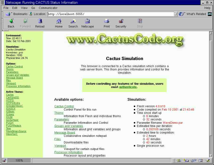
Click through the links to find information about the thorns, parameters and variables you are using. Go to the ViewPort and see Jpeg images from the simulation, if you press the refresh/reload button on your browser these will update (you may need to press e.g. the shift button as well depending on your browser and option settings), go to the Files page and see some of the output files that are being created. (If you have xgraph installed on your machine you can set up your browser to automatically view these when you click on them, see the WebBrowser-HOWTO for more details).

Viewing IsoSurfaces

Download IsoView the isosurface visualization client.

Start up IsoView, using IsoView -h <machine name> -dp 7051 -cp 7050

Again, this information can be found in the standard output, for example

INFO (IsoSurfacer): Isosurfacer listening for connections
                   host 'GridRebels-MacBook-Pro.local' control port 7050 data port 7051

You should now see rotating blobs appearing in the client, looking something like this

Now if you move the val slider, the value of the isosurface you see will change. Also, if you move the cursor in the main window, holding down the left, middle and right mouse buttons, the surface will rotate, translate and zoom.

Steering the Simulation

The web interface can also be used to control the simulation and to steer parameter values. Click on the Cactus Control link in the menu, and enter the user id anon and password anon (you can set these to be different values in the parameter file). Now you can pause, run or kill the simulation using the top buttons. If you are using the IsoView client press pause and see the blobs stop rotating/

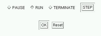
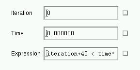
The buttons at the bottom allow you to pause the simulation at a given iteration number, or a given time, or when a condition is true. This is just a first version of a control interface, we hope it will become much more powerful, including many interactive debugging and collaborative tools.

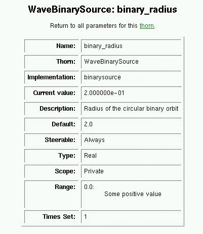
To steer simulation parameters, select Parameters from the menu, and then WaveBinarySource. We will change the parameter binary_radius, which sets the distance between the orbiting sources. Note that the parameters are divided into two sections, depending on whether they are steerable or not. This is decided by the thorn author.

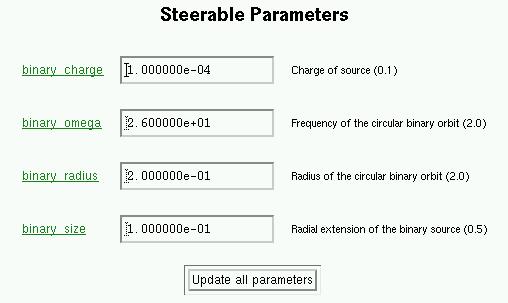
Note that if you click on the parameter name you get all the known information about that parameter.

Steer the parameter by changing the value in the box to zero, and pressing the update button. If you are watching the isosurfaces you should see the blobs move together. This can take a short while, since the isosurfaces are of the field and not the sources, and the field takes time to catch up.